Over the past decade, hardware has seen tremendous advances, from unified
memory that’s redefined how consumer GPUs work, to neural engines that can
run billion-parameter AI models on a laptop.
And yet, software is still slow, from seconds-long cold starts for
simple serverless functions, to hours-long ETL pipelines that merely
transform CSV files into rows in a database.
Back in 2011, a high-frequency trading engineer named Martin Thompson
noticed these issues, attributing
them
to a lack of Mechanical Sympathy. He borrowed this phrase from a Formula
1 champion:
You don’t need to be an engineer to be a racing driver, but you do need
Mechanical Sympathy.— Sir Jackie Stewart, Formula 1 World Champion
Although we’re not (usually) driving race cars, this idea applies to
software practitioners. By having “sympathy” for the hardware our software
runs on, we can create surprisingly performant systems. The
mechanically-sympathetic LMAX
Architecture processes
millions of events per second on a single Java thread.
Inspired by Martin’s work, I’ve spent the past decade creating
performance-sensitive systems, from AI inference platforms serving millions
of products at Wayfair, to novel binary encodings
that outperform Protocol Buffers.
In this article, I cover the principles of mechanical sympathy I use
every day to create systems like these – principles that can be applied most
anywhere, at any scale.
Not-So-Random Memory Access
Mechanical sympathy starts with understanding how CPUs store, access,
and share memory.
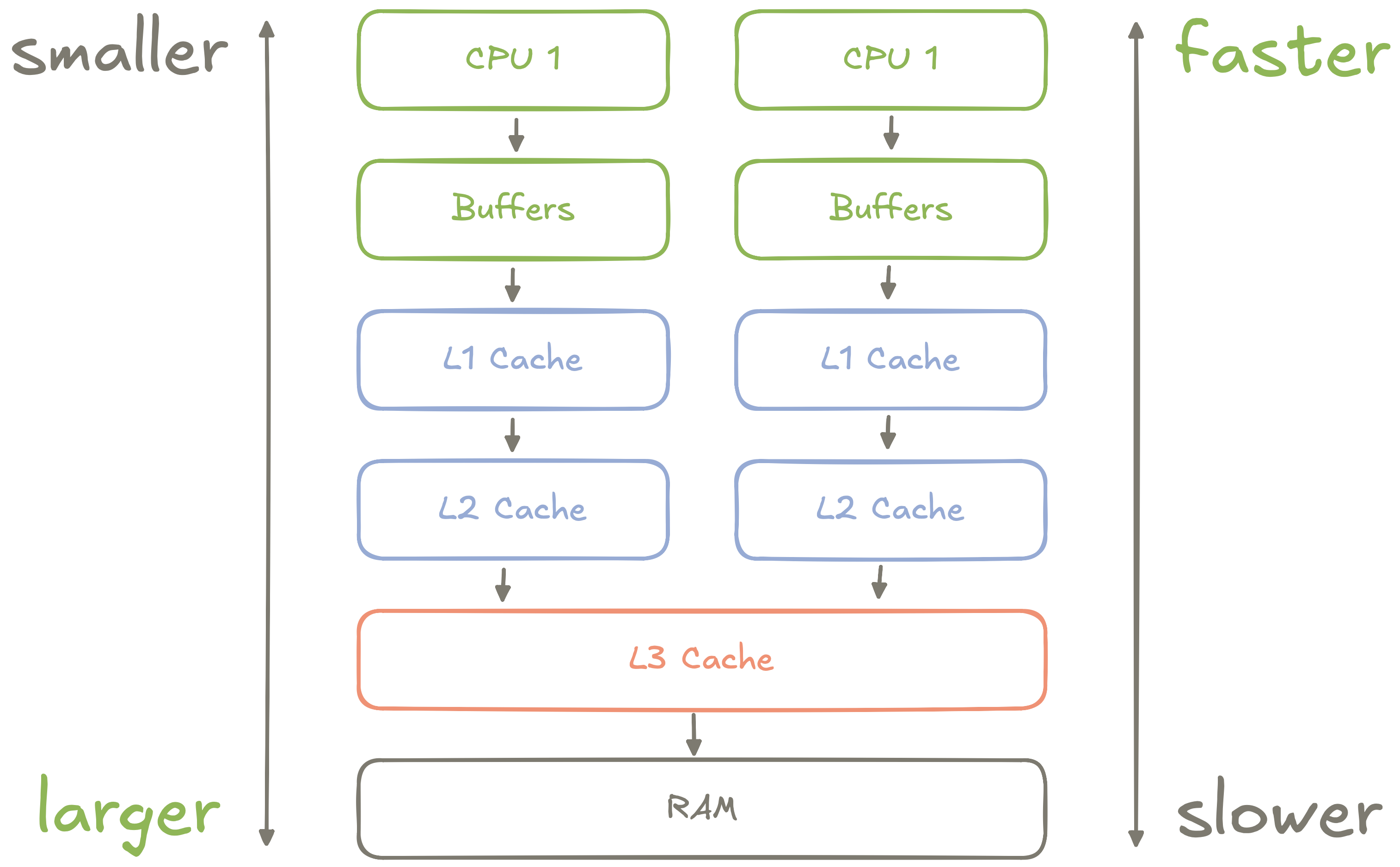
Figure 1: An abstract diagram of how CPU
memory is organized
Most modern CPUs – from Intel’s chips to Apple’s silicon – organize
memory into a hierarchy of registers, buffers, and
caches, each with different access latencies:
- Each CPU core has its own high-speed registers and buffers which are
used for storing things like local variables and in-flight instructions. - Each CPU core has its own Level 1 (L1) Cache which is much larger than
the core’s registers and buffers, but a little slower. - Each CPU core has its own Level 2 (L2) Cache which is even larger than
the L1 cache, and is used as a sort of buffer between the L1 and L3 caches. - Multiple CPU cores share a Level 3 (L3) Cache which is by far the
largest cache, but is much slower than the L1 or L2 caches. This cache is used
to share data between CPU cores. - All CPU cores share access to main memory, AKA RAM. This memory is, by
an order of magnitude, the slowest for a CPU to access.
Because CPUs’ buffers are so small, programs frequently need to access
slower caches or main memory. To hide the cost of this access, CPUs play a
betting game:
- Memory accessed recently will probably be accessed again soon.
- Memory near recently accessed memory will probably be accessed
soon. - Memory access will probably follow the same pattern.
In
practice,
these bets mean linear access outperforms access within the same
page, which in
turn vastly outperforms random access across pages.
Prefer algorithms and data structures that enable predictable,
sequential access to data. For example, when building an ETL pipeline,
perform a sequential scan over an entire source database and filter out
irrelevant keys instead of querying for entries one at a time by key.
Cache Lines and False Sharing
Within the L1, L2, and L3 caches, memory is usually stored in “chunks”
called Cache Lines. Cache lines are always a contiguous power of two
in length, and are often 64 bytes long.
CPUs always load (“read”) or store (“write”) memory in multiples of a
cache line, which leads to a subtle problem: What happens if two CPUs
write to two separate variables in the same cache line?
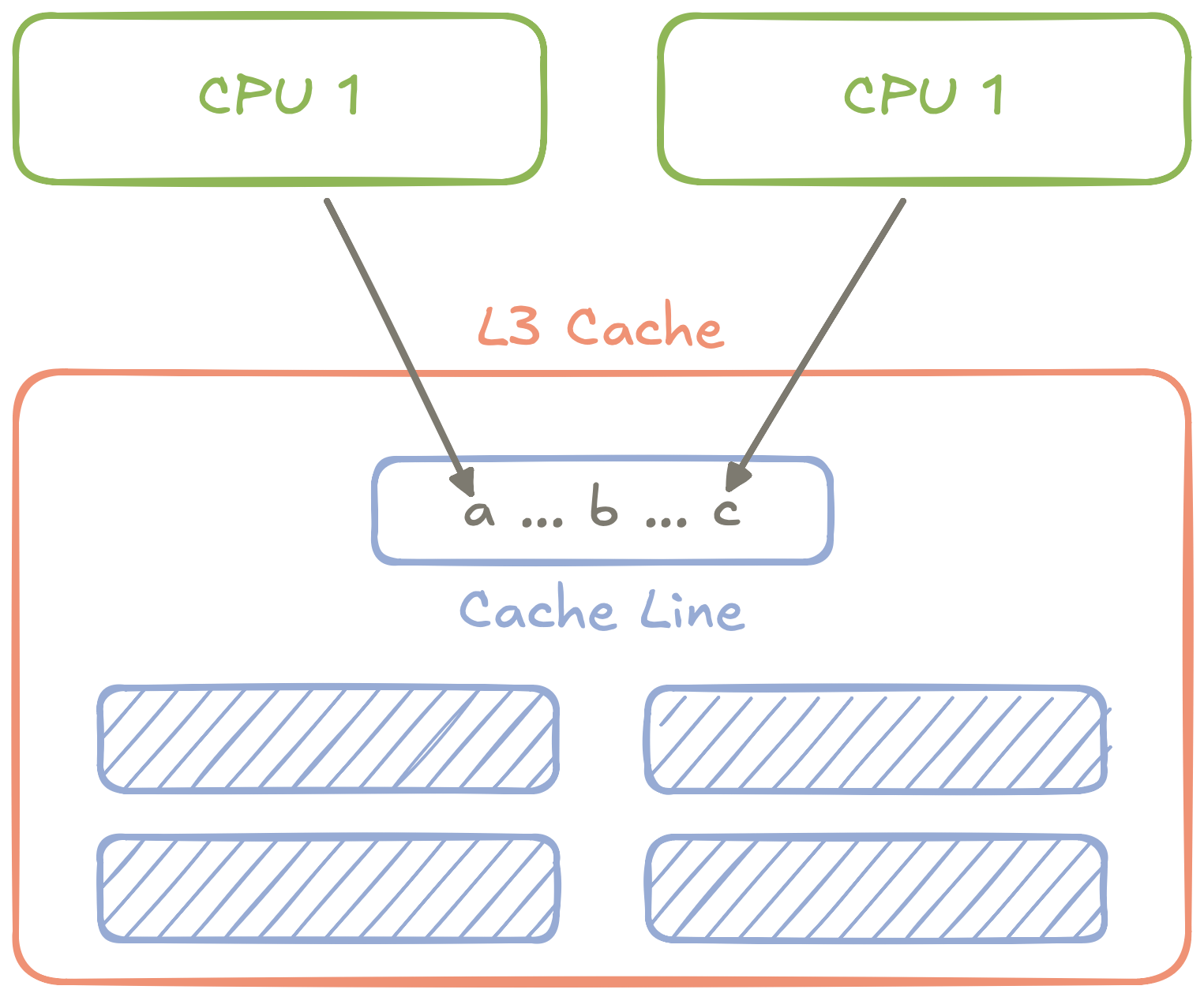
Figure 2: An abstract diagram of how two CPUs
accessing two different variables can still conflict if the variables are
in the same cache line.
You get False Sharing: Two CPUs fighting over access to two
different variables in the same cache line, forcing the CPUs to take
turns accessing the variables via the shared L3 cache.
To prevent false sharing, many low-latency applications will “pad”
cache lines with empty data so that each line effectively contains one
variable. The
difference
can be staggering:
- Without padding, cache line false sharing causes a near-linear increase in
latency as threads are added. - With padding, latency is nearly constant as threads are added.
Importantly, false sharing only appears when variables are being
written to. When they’re being read, each CPU can copy the cache line
to its local caches or buffers, and won’t have to worry about
synchronizing the state of those cache lines with other CPUs’ copies.
Because of this behavior, one of the most common victims of false
sharing is atomic variables. These are one of only a few data types (in
most languages) that can be safely shared and modified between threads
(and by extension, CPU cores).
If you’re chasing the final bit of performance in a
multithreaded application, check if there’s any data structure being
written to by multiple threads – and if that data structure might be a
victim of false sharing.
The Single Writer Principle
False sharing isn’t the only problem that arises when building
multithreaded systems. There are safety and correctness issues (like race
conditions), the cost of context-switching when threads outnumber CPU
cores, and the brutal overhead of mutexes
(“locks”).
These observations bring me to the mechanically-sympathetic principle I
use the most: The Single Writer
Principle.
In concept, the principle is simple: If there is some data (like an
in-memory variable) or resource (like a TCP socket) that an application
writes to, all of those writes should be made by a single thread.
Let’s consider a minimal example of an HTTP service that consumes text
and produces vector embeddings of that text. These embeddings would be
generated within the service via a text embedding AI model. For this
example, we’ll assume it’s an ONNX model, but Tensorflow, PyTorch, or any
other AI runtimes would work.
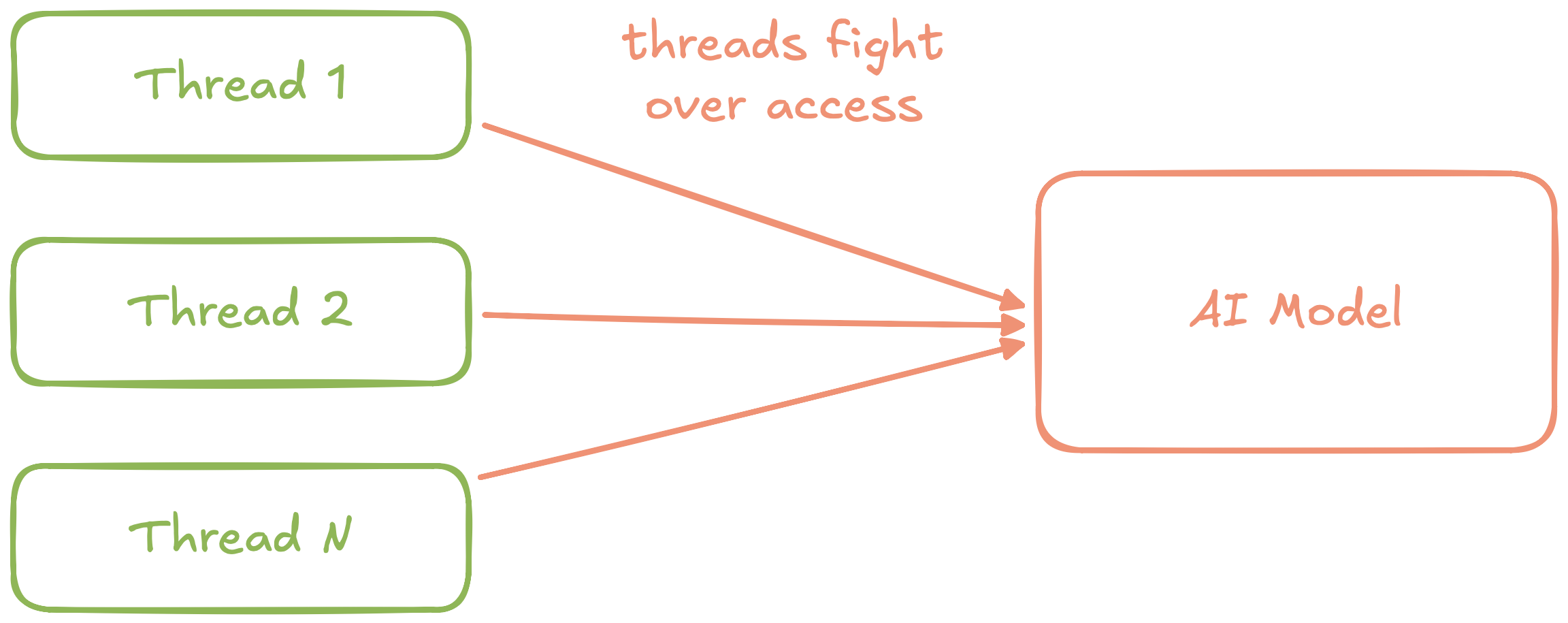
Figure 3: An abstract diagram of a naive text
embedding service
This service would quickly run into a problem: Most AI runtimes can
only execute one inference call to a model at a time. In the naive
architecture above, we use a mutex to work around this problem.
Unfortunately, if multiple requests hit the service at the same time,
they’ll queue for the mutex and quickly succumb to head-of-line
blocking.
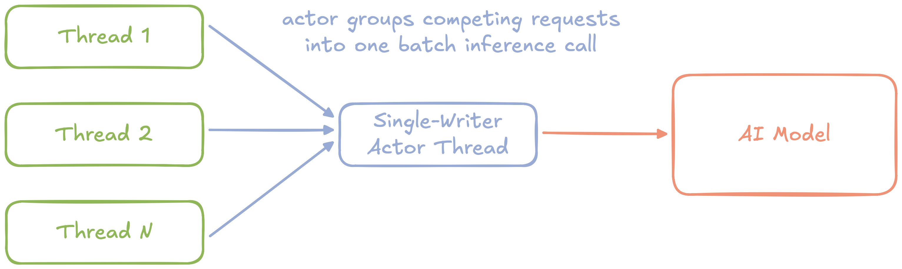
Figure 4: An abstract diagram of a text embedding
service using the single-writer principle with batching
We can eliminate these issues by refactoring with the single-writer
principle. First, we can wrap access to the model in a dedicated
Actor thread. Instead of
request threads competing for a mutex, they now send asynchronous messages
to the actor.
Because the actor is the single-writer, it can group independent
requests into a single batch inference call to the underlying model, and
then asynchronously send the results back to individual request
threads.
Avoid protecting writable resources with a mutex. Instead, dedicate a single thread (“actor”) to own every write, and use asynchronous messaging to submit writes from other threads to the actor.
Natural Batching
Using the single-writer principle, we’ve removed the mutex from our
simple AI service, and added support for batch inference calls. But how
should the actor create these batches?
If we wait for a predetermined batch size, requests could block for
an unbounded amount of time until enough requests come in. If we create
batches at a fixed interval, requests will block for a bounded amount of
time between each batch.
There’s a better way than either of these approaches: Natural Batching.
With natural batching, the actor begins creating a batch as soon as
requests are available in its queue, and completes the batch as soon as
the maximum batch size is reached or the queue is empty.
Borrowing a worked example from Martin’s original post on natural
batching, we can see how it amortizes per-request latency over time:
| Strategy | Best (µs) | Worst (µs) |
|---|---|---|
| Timeout | 200 | 400 |
| Natural | 100 | 200 |
This example assumes each batch has a fixed latency of 100µs.
With a timeout-based batching strategy, assuming a timeout of 100µs,
the best-case latency will be 200µs when all requests in the batch are
received simultaneously (100µs for the request itself, and 100µs
waiting for more requests before sending a batch). The worst-case latency
will be 400µs when some requests are received a little late.
With a natural batching strategy, the best-case latency will be 100µs
when all requests in the batch are received simultaneously. The worst-case
latency will be 200µs when some requests are received a little late.
In both cases, the performance of natural batching is twice as good as a
timeout-based strategy.
If a single writer handles batches of writes (or reads!), build each batch greedily: Start the batch as soon as data is available, and finish when the queue of data is empty or the batch is full.
These principles work well for individual apps, but they scale to
entire systems. Sequential, predictable data access applies to a big data
lake as much as an in-memory array. The single-writer principle can boost
performance of an IO-intensive app, or provide a strong foundation for a
CQRS architecture.
When we write software that’s mechanically sympathetic, performance
follows naturally, at every scale.
But before you go: prioritize observability before optimization.
You can’t improve what you can’t measure. Before applying any of these
principles, define your SLIs, SLOs, and
SLAs so you know where to focus and
when to stop.
Prioritize observability before optimization, before applying
these principles, measure performance and understand your goals.


Speak Your Mind